Amperes Law -Definition, Statement, Examples, Equation, FAQs

Ampere’s circuital equation in electromagnetism integrates the magnetic field around a closed loop with electric current passing through it. This article will help us understand more about Ampere circuital laws. In this article we will discuss what is Ampere's circuital law, Ampere's law equation, Ampere's circuital law derivation using Bio-savarts law, application of Ampere's circuital law and Maxwell Ampere circuital law

State Ampere’s Law

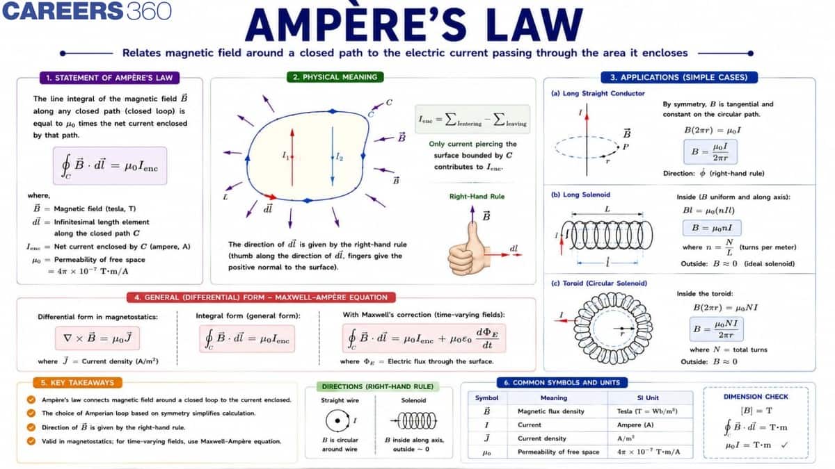
“The magnetic field produced by an electric current is proportional to its magnitude, with proportionality constant equal to permeability of empty space.”

According to Ampere circuital law, magnetic fields are related to the electric current created in them. The law specifies the magnetic field is associated with a particular current or vice versa as long as the electric field remains constant.

Who Was Andre-Marie Ampere?

André-Marie Ampère was a scientist who experimented with current-carrying wires and forces acting on them. The experiment took place in the late 1820s, during the time Faraday was developing his Faraday's Law. Faraday and Amperes law had no notion that their work would be integrated four years later by Maxwell himself.

Ampere’s Circuital Law

The line integral of the magnetic field surrounding a closed loop equals the algebraic total of currents going through the loop, according to Ampere circuital law's circuital equation.

Ampere's Circuital Law Formula

If a conductor is carrying current I, the current flow generates a magnetic field around the wire. Ampere's circuital law formula is given as:

$$\int \mathrm{B} \cdot \mathrm{dl}=\mu_o I$$

• where,
• $\int \mathrm{B} \cdot \mathrm{dl}$ is the line integral of B in a closed path
• $\mu$ is the permeability of free space
• $I$ is the current enclosed

The left side of the equation states that if an imaginary path encircles the wire and the magnetic field is added at each point, the current surrounded by this path, as represented by the current enclosed, is numerically equivalent to the current encircled by this route.

Also read -

• NCERT Solutions for Class 11 Physics
• NCERT Solutions for Class 12 Physics
• NCERT Solutions for All Subjects

Ampere's Circuital Law Derivation From Bio-Savart Law

The Bio-savart law is given as

$d \vec{B}=\frac{\mu_0}{4 \pi} \frac{I d \vec{l} \times \hat{r}}{r^2}$

Integrating on both sides,

$\vec{B}=\frac{\mu_0}{4 \pi} \int \frac{I d \vec{l} \times \hat{r}}{r^2}$

Take the line integral of the equation

$\oint \vec{B} \cdot d \vec{l}=\oint\left(\frac{\mu_0}{4 \pi} \int \frac{I d \vec{l}^{\prime} \times \hat{r}}{r^2}\right) \cdot d \vec{l}$

Simplify the integral

$\oint \vec{B} \cdot d \vec{l}=\frac{\mu_0}{4 \pi} \int\left(I d \vec{l} \times \oint \frac{\hat{r}}{r^2} \cdot d \vec{l}\right)$

Stoke's theorem states that the surface integral of the curl of a vector field is equal to the line integral of the field along that boundary. Applying Stoke's theorem on the above equation we get,

$\oint \vec{B} \cdot d \vec{l}=\mu_0 I_{\mathrm{enc}}$

This is the Ampere's law equation

Maxwell-Ampere Circuital Law

It is an extension of Ampere's law. It states that an electric current or changing electric flux passing through a surface generates a rotating magnetic field around any boundary path.

$\nabla \times \mathbf{B}=\mu_0 \mathbf{J}+\mu_0 \epsilon_0 \frac{\partial \mathbf{E}}{\partial t}$

where,

$\nabla \times \mathbf{B}$ is the curl of magnetic field

$\mu_0$ is the permeability of free space

$J$ is the current density

$\epsilon_0$ is the permittivity of free space

${\partial \mathbf{E}}{\partial t}$ is the time rate of change of electric field

Application of Ampere’s Circuital Law

Ampere circuital law and its applications are given :

1. Determine the magnetic induction that occurs when a long current-carrying wire is used.

2. To find the magnetic field inside a toroid, use the ampere circuital law.

3. Calculate the magnetic field that a long current-carrying conducting cylinder generates.

4. The magnetic field inside the conductor must be determined.

5. Find the forces that exist between currents.

Ampere Circuital Law’s Circuital Law and Magnetic Field

Since its creation, Ampere circuital law has acquired popularity due to its practicality. It has also been used in real-life settings. The production of machines is one of the most well-known platforms where Ampere circuital law is often applied.

Motors, generators, transformers, and similar devices are examples of machinery. All of these are based on the concepts of ampere circuital law application. Comprehending these concepts is critical, especially since they are required at higher levels of education. These ideas form the foundation for some of the most important derivations and principles in physics.

The following is a list of applications in which Ampere circuital law's circuital law is used to find the magnetic field:

1. Solenoid

2. The straight wire

3. The wire is thick

4. Conductor in the shape of a cylinder

5. solenoid with a toroidal shape

It's worth noting that, even though the law's application varies widely, the working premise of the law stays the same throughout each phase. It is the operating principle of a wide range of machinery and devices, and it is frequently used as a component of other devices.